
JOURNAL OF NATURAL RESOURCES >
Spatio-temporal evolution and spatial interaction of regional eco-efficiency in China
Received date: 2019-12-14
Request revised date: 2020-02-19
Online published: 2020-11-27
Copyright
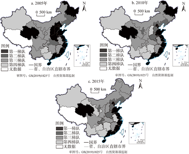
Eco-efficiency is an important indicator for measuring sustainable development. Clarifying the spatial distribution of eco-efficiency and its evolution is of vital importance to achieving coordinated regional development of China's economy and environment. However, previous research has failed to consider the spatial interaction distribution of eco-efficiency. The SBM model considering undesired output was used to measure the eco-efficiency of 30 provinces (municipalities and autonomous regions) in China from 2005 to 2015, and the spatial econometric model was used to investigate the spatial interaction pattern of eco-efficiency in China. The results show that: (1) From the perspective of the whole country or by region, China's eco-efficiency has generally shown a downward trend. (2) From the perspective of the evolution of the spatial distribution of eco-efficiency, the characteristics of high eco-efficiency distributed in developed provinces have been continuously strengthened, and low eco-efficiency areas are mainly distributed in developing provinces. Beijing, Tianjin, Shandong, Jiangsu, Shanghai, Zhejiang, Fujian, Guangdong, Hainan, Qinghai have always been in the first echelon of eco-efficiency, while Xinjiang, Guangxi and Hunan have always been in the fourth echelon. From 2005 to 2015, the members of each echelon changed, but the distribution characteristics based on the level of economic development remained basically unchanged. (3) At the national level, the estimation results based on the economic weight matrix show that there is a positive spatial interaction effect of eco-efficiency among regions. The improvement of eco-efficiency in a certain region will have a positive spillover effect on its economic neighbors. Extensive learning sharing and competition among different regions may explain the positive eco-efficiency interactions among regions. (4) The sub-sample test shows that the eco-efficiency of developed and developing regions shows a positive spatial interaction effect, and the spatial interaction effect is greater than the spatial interaction effect between the two types of regions, indicating that the distribution in China's eco-efficiency is based on the level of economic development, thus showing the "sorting" based on the level of economic development. This conclusion is still robust even with the geographic distance and adjacent weight matrix.
SHEN Wei-teng , HU Qiu-guang , LI Jia-lin , CHEN Qi . Spatio-temporal evolution and spatial interaction of regional eco-efficiency in China[J]. JOURNAL OF NATURAL RESOURCES, 2020 , 35(9) : 2149 -2162 . DOI: 10.31497/zrzyxb.20200909
Table 1 The indicators used to measure eco-efficiency表1 生态效率测算所采用的指标 |
| 类别 | 指标 | 单位 |
|---|---|---|
| 投入 | 固定资本形成总额 | 亿元 |
| 年底就业人数 | 万人 | |
| 建设用地供应 | hm2 | |
| 能源消费量 | 万t标准煤 | |
| 水资源利用 | 亿m3 | |
| 非期望产出 | 废水排放总量 | 万t |
| 化学需氧量 | 万t | |
| SO2排放量(粉) 烟尘排放量 | 万t | |
| 万t | ||
| 期望产出 | 实际地区生产总值 | 亿元 |
Table 2 Variable definitions表2 变量定义 |
| 变量 | 计算方法 | 单位 |
|---|---|---|
| 第三产业占比 | 第三产业产值/地区生产总值 | % |
| 人均GDP | 实际GDP/总人口数 | 元/人 |
| 贸易开放程度 | 进出口总额/地区生产总值 | % |
| 城镇化水平 | 年末城镇人口/总人口数 | % |
| 能源使用强度 | 能源消费总量/实际工业增加值 | 标准煤/万元 |
| 政府对环境的管制 | 排污费缴纳总额/缴纳企业个数 | 万元/个 |
| 公众对环境的关注 | 因环境污染来信总数/总人口 | 封/万人 |
| 公民受教育水平 | 大专及以上学历人数占比 | % |
Table 3 The regional eco-efficiency in China from 2005 to 2015表3 2005—2015年中国区域生态效率测算结果 |
| 地区/年份 | 2005 | 2006 | 2007 | 2008 | 2009 | 2010 | 2011 | 2012 | 2013 | 2014 | 2015 | 均值 |
|---|---|---|---|---|---|---|---|---|---|---|---|---|
| 北京 | 1.000 | 1.000 | 1.000 | 1.000 | 1.000 | 1.000 | 1.000 | 1.000 | 1.000 | 1.000 | 1.000 | 1.000 |
| 天津 | 1.000 | 1.000 | 1.000 | 1.000 | 1.000 | 1.000 | 1.000 | 1.000 | 1.000 | 1.000 | 1.000 | 1.000 |
| 河北 | 1.000 | 1.000 | 0.556 | 0.480 | 0.499 | 0.500 | 0.442 | 0.427 | 0.407 | 0.409 | 0.421 | 0.558 |
| 福建 | 1.000 | 1.000 | 1.000 | 1.000 | 1.000 | 1.000 | 1.000 | 1.000 | 1.000 | 0.474 | 1.000 | 0.952 |
| 内蒙古 | 1.000 | 1.000 | 1.000 | 0.349 | 1.000 | 0.412 | 0.410 | 1.000 | 0.353 | 0.363 | 0.375 | 0.660 |
| 辽宁 | 0.500 | 0.427 | 0.397 | 0.402 | 0.485 | 0.507 | 0.421 | 0.440 | 0.478 | 0.446 | 0.458 | 0.451 |
| 吉林 | 0.474 | 0.391 | 0.384 | 0.363 | 0.375 | 0.355 | 0.356 | 0.393 | 0.391 | 0.367 | 0.377 | 0.384 |
| 黑龙江 | 1.000 | 1.000 | 1.000 | 1.000 | 1.000 | 1.000 | 0.381 | 0.358 | 0.358 | 0.396 | 0.401 | 0.718 |
| 上海 | 1.000 | 1.000 | 1.000 | 1.000 | 1.000 | 1.000 | 1.000 | 1.000 | 1.000 | 1.000 | 1.000 | 1.000 |
| 江苏 | 1.000 | 1.000 | 1.000 | 1.000 | 1.000 | 1.000 | 1.000 | 1.000 | 1.000 | 1.000 | 1.000 | 1.000 |
| 浙江 | 1.000 | 1.000 | 1.000 | 1.000 | 1.000 | 1.000 | 1.000 | 1.000 | 1.000 | 1.000 | 1.000 | 1.000 |
| 山东 | 1.000 | 1.000 | 1.000 | 1.000 | 1.000 | 1.000 | 1.000 | 1.000 | 1.000 | 1.000 | 1.000 | 1.000 |
| 湖北 | 0.592 | 0.515 | 0.400 | 0.377 | 0.406 | 0.364 | 0.326 | 0.321 | 0.344 | 0.354 | 0.371 | 0.397 |
| 广东 | 1.000 | 1.000 | 1.000 | 1.000 | 1.000 | 1.000 | 1.000 | 1.000 | 1.000 | 1.000 | 1.000 | 1.000 |
| 重庆 | 0.386 | 0.376 | 0.383 | 0.386 | 0.361 | 0.374 | 0.371 | 0.415 | 0.417 | 0.411 | 0.440 | 0.393 |
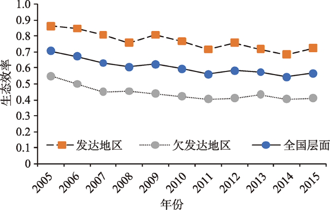
| 发达地区均值 | 0.863 | 0.847 | 0.808 | 0.757 | 0.808 | 0.767 | 0.714 | 0.757 | 0.717 | 0.681 | 0.723 | 0.767 |
| 江西 | 0.434 | 0.419 | 0.368 | 0.394 | 0.340 | 0.342 | 0.307 | 0.327 | 0.306 | 0.324 | 0.319 | 0.353 |
| 河南 | 1.000 | 0.540 | 0.470 | 0.446 | 0.460 | 0.450 | 0.439 | 0.400 | 0.425 | 0.444 | 0.437 | 0.501 |
| 湖南 | 0.433 | 0.468 | 0.368 | 0.336 | 0.358 | 0.301 | 0.274 | 0.267 | 0.279 | 0.283 | 0.301 | 0.333 |
| 山西 | 0.489 | 0.449 | 0.364 | 0.381 | 0.335 | 0.315 | 0.286 | 0.300 | 0.291 | 0.301 | 0.316 | 0.348 |
| 广西 | 0.380 | 0.350 | 0.287 | 0.297 | 0.272 | 0.248 | 0.240 | 0.240 | 0.249 | 0.254 | 0.262 | 0.280 |
| 海南 | 1.000 | 1.000 | 1.000 | 1.000 | 1.000 | 1.000 | 1.000 | 1.000 | 1.000 | 1.000 | 1.000 | 1.000 |
| 安徽 | 0.505 | 0.428 | 0.362 | 0.340 | 0.352 | 0.337 | 0.298 | 0.286 | 0.281 | 0.283 | 0.290 | 0.342 |
| 四川 | 0.445 | 0.433 | 0.342 | 0.337 | 0.362 | 0.347 | 0.336 | 0.348 | 0.371 | 0.363 | 0.362 | 0.368 |
| 贵州 | 0.438 | 0.393 | 0.329 | 0.361 | 0.313 | 0.291 | 0.286 | 0.273 | 0.262 | 0.260 | 0.257 | 0.315 |
| 云南 | 0.446 | 0.388 | 0.335 | 0.345 | 0.295 | 0.276 | 0.241 | 0.258 | 0.235 | 0.218 | 0.231 | 0.297 |
| 陕西 | 0.440 | 0.427 | 0.390 | 0.373 | 0.361 | 0.346 | 0.356 | 0.327 | 0.322 | 0.326 | 0.350 | 0.365 |
| 甘肃 | 0.389 | 0.406 | 0.435 | 0.380 | 0.329 | 0.358 | 0.299 | 0.329 | 0.287 | 0.289 | 0.287 | 0.344 |
| 青海 | 1.000 | 1.000 | 1.000 | 1.000 | 1.000 | 1.000 | 1.000 | 1.000 | 1.000 | 1.000 | 1.000 | 1.000 |
| 宁夏 | 0.508 | 0.480 | 0.423 | 0.477 | 0.468 | 0.460 | 0.474 | 0.585 | 1.000 | 0.534 | 0.573 | 0.544 |
| 新疆 | 0.360 | 0.322 | 0.314 | 0.347 | 0.337 | 0.290 | 0.276 | 0.228 | 0.202 | 0.203 | 0.199 | 0.280 |
| 欠发达地区均值 | 0.551 | 0.500 | 0.452 | 0.454 | 0.439 | 0.424 | 0.407 | 0.411 | 0.434 | 0.405 | 0.412 | 0.444 |
| 总体均值 | 0.707 | 0.674 | 0.630 | 0.606 | 0.624 | 0.596 | 0.561 | 0.584 | 0.575 | 0.543 | 0.568 | 0.606 |
Fig. 1 The variation of regional eco-efficiency in China from 2005 to 2015图1 2005—2015年中国区域生态效率变化情况 |
Fig. 2 The distribution and evolution of regional eco-efficiency in China图2 中国区域生态效率分布及其演变状况 |
Table 4 The estimation results based on national data表4 基于全国数据的估计结果 |
| 变量 | (1) | (2) | (4) | (3) |
|---|---|---|---|---|
| OLS | 经济权重 | 地理权重 | 相邻权重 | |
| 空间滞后项系数 | — | 0.2216*** | 0.0747 | 0.0973 |
| — | (0.0851) | (0.1580) | (0.0719) | |
| 政府对环境的规制 | -0.0072*** | -0.0075*** | -0.0073*** | -0.0071*** |
| (0.0025) | (0.0024) | (0.0024) | (0.0024) | |
| 公众对环境的关注 | 0.0089 | 0.0094* | 0.0089 | 0.0085 |
| (0.0056) | (0.0054) | (0.0055) | (0.0055) | |
| 人均GDP | -0.1350*** | -0.1164*** | -0.1286*** | -0.1218*** |
| (0.0357) | (0.0353) | (0.0377) | (0.0363) | |
| 人均GDP平方项 | 0.0014 | 0.0012 | 0.0014 | 0.0015 |
| (0.0020) | (0.0019) | (0.0019) | (0.0019) | |
| 贸易开放程度 | -0.1258* | -0.1191* | -0.1266* | -0.1216* |
| (0.0682) | (0.0661) | (0.0671) | (0.0669) | |
| 城镇化率 | 0.0004 | 0.0005 | 0.0003 | -0.0004 |
| (0.0039) | (0.0038) | (0.0039) | (0.0039) | |
| 第三产业占比 | 0.0018 | 0.0012 | 0.0018 | 0.0017 |
| (0.0024) | (0.0023) | (0.0024) | (0.0024) | |
| 能源使用强度 | -0.0331*** | -0.0307** | -0.0335*** | -0.0347*** |
| (0.0127) | (0.0124) | (0.0126) | (0.0126) | |
| 公民受教育水平 | 0.0022 | 0.0027 | 0.0023 | 0.0024 |
| (0.0025) | (0.0024) | (0.0025) | (0.0024) | |
| R2 | 0.2326 | 0.2318 | 0.2327 | 0.2361 |
| 观测值 | 330 | 300 | 300 | 300 |
注:***、**和*分别为在1%、5%和10%的显著性水平上显著,括号内为标准误,下同;“—”表示此项为空。 |
Table 5 The estimation results based on the subsample表5 分样本估计结果 |
| 变量 | 经济权重 | 地理权重 | 相邻权重 | |||||
|---|---|---|---|---|---|---|---|---|
| (5) | (6) | (7) | (8) | (9) | (10) | |||
| 发达地区 | 欠发达地区 | 发达地区 | 欠发达地区 | 发达地区 | 欠发达地区 | |||
| 空间滞后项系数 | 0.4354*** | 0.6159*** | 0.6036*** | 0.7072*** | 0.3127*** | 0.4988*** | ||
| (0.0905) | (0.0630) | (0.0924) | (0.0658) | (0.0673) | (0.0686) | |||
| 控制变量 | 有 | 有 | 有 | 有 | 有 | 有 | ||
| R2 | 0.1357 | 0.3179 | 0.1154 | 0.3507 | 0.1622 | 0.2586 | ||
| 观测值 | 150 | 150 | 150 | 150 | 150 | 150 | ||
注:受篇幅所限,未包括控制变量估计结果。 |
| [1] |
|
| [2] |
|
| [3] |
|
| [4] |
|
| [5] |
This paper presents the eco-efficiency of energy intensity, material consumption, water use, waste generation, and CO2 emission in terms of production value in net sales (US$) per environmental influence using empirical evaluation. Evaluation has been considered only within production process boundary of iron rod industry. Evaluation of eco-efficiency tried to couple the economic and environmental influences of industry to know economic and environmental excellence. Eco-efficiency of iron rod industry was quantitatively analyzed and determined that energy, material consumption, water use, waste generation, and CO2 emission eco-efficiency have been increased gradually along with increased production during analysis period of five years (2001–2005). It was possible due to installing heat recovery unit along with innovative processes modification. While comparing each year's eco-efficiency of all above-mentioned parameters, eco-efficiencies were increased that indicates less resource use and less waste released. As a general statement of overall comparison and characterization of eco-efficiencies of five years duration, iron rod industry was eco-efficient in all aspects. Eco-efficiency being an emerging trend has not yet been implemented in Nepal. It is further recommended to adopt the eco-efficiency evaluation in other industries. In addition, it is high time to augment the provision of eco-efficiency concepts in industrial policy and legislation concerned. ]]> |
| [6] |
[
|
| [7] |
|
| [8] |
|
| [9] |
[
|
| [10] |
|
| [11] |
|
| [12] |
|
| [13] |
[
|
| [14] |
|
| [15] |
|
| [16] |
[
|
| [17] |
|
| [18] |
[
|
| [19] |
[
|
| [20] |
[
|
| [21] |
[
|
| [22] |
|
| [23] |
|
| [24] |
[
|
| [25] |
[
|
| [26] |
[
|
| [27] |
|
| [28] |
[
|
| [29] |
|
| [30] |
The literature on trade openness, economic development, and the environment is largely inconclusive about the environmental consequences of trade. This study treats trade and income as endogenous and estimates the overall impact of trade openness on environmental quality using the instrumental variables technique. We find that whether or not trade has a beneficial effect on the environment varies depending on the pollutant and the country. Trade is found to benefit the environment in OECD countries. It has detrimental effects, however, on sulfur dioxide (SO2) and carbon dioxide (CO2) emissions in non-OECD countries, although it does lower biochemical oxygen demand (BOD) emissions in these countries. We also find the impact is large in the long term, after the dynamic adjustment process, although it is small in the short term. ]]> |
| [31] |
|
| [32] |
[
|
| [33] |
|
| [34] |
|
| [35] |
[
|
| [36] |
|
| [37] |
|
| [38] |
[
|
| [39] |
|
/
| 〈 |
|
〉 |