
贫困的“物以类聚”:中国的农村空间贫困陷阱及其识别
罗翔(1978- ),男,江西九江人,博士,副教授,研究方向为区域经济学与发展经济学。E-mail: philiplaw@163.com
收稿日期: 2019-04-30
要求修回日期: 2019-08-20
网络出版日期: 2020-12-28
基金资助
国家自然科学基金项目(71974071,71774066,71904151)
中央高校基本科研业务经费“土地利用与粮食安全”青年学术创新团队项目(CCNU19TD004)
"Birds of a feather flock together":China's rural spatial poverty trap and its identification
Received date: 2019-04-30
Request revised date: 2019-08-20
Online published: 2020-12-28
Copyright
理解贫困陷阱及其成因是理解减贫机制,进而理解贫困治理的基础。早期的实证研究注重从收入的角度研究农村贫困,较新的研究开始关注“空间外部性”对农村贫困的影响。然而,要正确识别农村的“贫困陷阱”,就需要对上述两个维度同时进行解释。鉴于此,运用中国县级层面的面板数据,从聚集与持久两个维度对中国的农村贫困陷阱进行了识别。研究结果表明:2006—2016年,中国农村的贫困空间格局几乎没有变化,并且贫困的空间分布与经济增长也并非是同步的,贫困县的分布主要与地形(坡度、海拔)因素有关;进一步研究还发现,中国的农村贫困具有持久性,贫困县收入存在低水平的均衡,贫困县与非贫困县之间存在收入的“俱乐部收敛”。本文揭示了空间外部性与农村贫困之间的关系,为正确评估经济发展与扶贫开发,合理制定区域反贫困瞄准机制提供了支持。
罗翔 , 李崇明 , 万庆 , 张祚 . 贫困的“物以类聚”:中国的农村空间贫困陷阱及其识别[J]. 自然资源学报, 2020 , 35(10) : 2460 -2472 . DOI: 10.31497/zrzyxb.20201012
Examining the poverty trap and its causes is the basis for understanding the mechanism of poverty reduction and governance. Current research no longer confines rural poverty to "insufficient capital formation", but emphasizes the importance of spatial factors. Based on the panel data at the county level, this paper identifies the rural poverty trap in China from two dimensions of aggregation and persistence. This study shows that the spatial pattern of poverty in rural China remained almost unchanged during 2006-2016, and the spatial distribution of poverty is not synchronized with economic growth. The distribution of poverty-stricken counties is mainly related to terrain conditions (slope, elevation). Further research also finds that rural poverty in China is persistent. There is a low level equilibrium of income in poverty-stricken counties, and there is a "club convergence" between poverty-stricken and non-poverty-stricken counties. This study reveals the relationship between spatial externalities and rural poverty, which provides support for the correct assessment of economic development and poverty alleviation, and the rational formulation of regional anti-poverty targeting mechanism.
Key words: space; aggregation; persistence; poverty trap
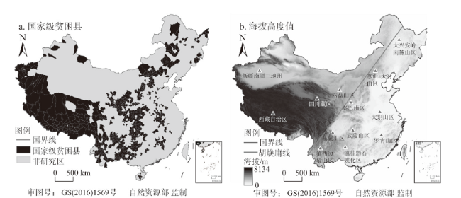
Fig. 1 Spatial distribution characteristics of rural poverty in China图1 中国农村贫困的空间分布特征 |
Fig. 2 Spatio-temporal distribution characteristics of China's poor population图2 中国贫困人口的时空分布特征 |
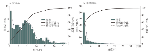
Fig. 3 Distribution frequency of poverty-stricken counties and non-poverty counties on different slopes图3 不同坡度下贫困县与非贫困县的分布频率 |
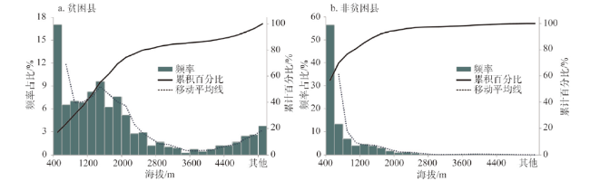
Fig. 4 Distribution frequency of poverty-stricken counties and non-poverty counties at different altitudes图4 不同海拔下贫困县与非贫困县的分布频率 |
Fig. 5 Possibility of poverty trap and convergence diagram图5 贫困陷阱可能性与收敛示意图 |
Table 1 Persistent grouping regression results of poverty表1 贫困的持久性分组回归结果 |
| 被解释变量:对数形式的农村人均纯收入 | |||
|---|---|---|---|
| 模型1:OLS | 模型2:FE | 模型3:拟差分[19] | |
| 面板A:贫困县 | |||
| 滞后1期对数形式的农村人均纯收入 | 0.830*** (0.028) | 0.701*** (0.004) | 0.752*** (0.060) |
| 滞后1期对数形式的农村人均纯收入的平方 | 0.010*** (0.003) | 0.039*** (0.005) | 0.039*** (0.011) |
| 滞后1期对数形式的农村人均纯收入的立方 | -0.001*** (0.000) | -0.003*** (0.000) | -0.003*** (0.000) |
| 控制变量 | 控制 | 控制 | 控制 |
| 异方差 | 控制 | 控制 | 控制 |
| 时间固定效应 | 控制 | 控制 | 控制 |
| 个体固定效应 | 未控制 | 控制 | 控制 |
| Hausman检验(P值) | 0.000 | ||
| F检验(P值) | 0.000 | ||
| R2 | |||
| 观察值 | 8880 | 8880 | 8288 |
| 面板B:非贫困县 | |||
| 滞后1期对数形式的农村人均纯收入 | 0.612*** (0.033) | 0.701*** (0.044) | 0.804*** (0.257) |
| 滞后1期对数形式的农村人均纯收入的平方 | 0.024*** (0.011) | 0.004 (0.069) | -0.003 (0.032) |
| 滞后1期对数形式的农村人均纯收入的立方 | -0.000 (0.004) | -0.002 (0.004) | -0.002 (0.003) |
| 控制变量 | 控制 | 控制 | 控制 |
| 异方差 | 控制 | 控制 | 控制 |
| 个体固定效应 | 控制 | 控制 | 控制 |
| 时间固定效应 | 未控制 | 控制 | 控制 |
| Hausman检验(P值) | |||
| F检验(P值) | 0.000 | ||
| R2 | 0.993 | 0.988 | 0.855 |
| 观察值 | 25920 | 25920 | 24192 |
注:*、**、***分别表示在10%、5%、1%的置信水平下显著不为0;括号中报告的是标准误,下同。 |
Table 2 Regression results of poverty club convergence表2 贫困的俱乐部收敛回归结果 |
| 被解释变量:农村人均纯收入的增长率 | |||
|---|---|---|---|
| 模型1:OLS | 模型2:FE | 模型3:拟差分[19] | |
| 面板A:贫困县 | |||
| 滞后1期对数形式的农村人均纯收入 | -15.889*** (0.347) | -14.107*** (0.656) | -88.704*** (20.572) |
| 控制变量 | 控制 | 控制 | 控制 |
| 异方差 | 控制 | 控制 | 控制 |
| 时间固定效应 | 控制 | 控制 | 控制 |
| 个体固定效应 | 未控制 | 控制 | 控制 |
| Hausman检验(P值) | 0.000 | ||
| F检验(P值) | 0.018 | ||
| R2 | 0.187 | 0.202 | 0.263 |
| 观察值 | 8880 | 8880 | 8288 |
| 面板B:非贫困县 | |||
| 滞后1期对数形式的农村人均纯收入 | -6.604*** (0.200) | -14.772*** (1.049) | -55.443*** (7.282) |
| 控制变量 | 控制 | 控制 | 控制 |
| 异方差 | 控制 | 控制 | 控制 |
| 个体固定效应 | 控制 | 控制 | 控制 |
| 时间固定效应 | 未控制 | 控制 | 控制 |
| Hausman检验(P值) | 0.000 | ||
| F检验(P值) | 0.000 | ||
| R2 | 0.127 | 0.102 | 0.407 |
| 观察值 | 25920 | 25920 | 24192 |
| 面板C:全样本 | |||
| 滞后1期对数形式的农村人均纯收入 | -3.116 (7.112) | -1.157 (1.886) | -74.220 (63.113) |
| 控制变量 | 控制 | 控制 | 控制 |
| 异方差 | 控制 | 控制 | 控制 |
| 个体固定效应 | 控制 | 控制 | 控制 |
| 时间固定效应 | 未控制 | 控制 | 控制 |
| Hausman检验(P值) | 0.000 | ||
| F检验(P值) | 0.000 | ||
| R2 | 0.160 | 0.114 | 0.326 |
| 观察值 | 34000 | 34000 | 32480 |
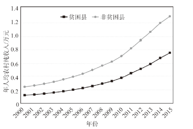
Fig. 6 Trends in annual per capita rural net income in poor and non-poverty counties图6 贫困县与非贫困县年人均农村纯收入的变动趋势 |
| [1] |
[
|
| [2] |
|
| [3] |
|
| [4] |
|
| [5] |
|
| [6] |
|
| [7] |
|
| [8] |
|
| [9] |
[
|
| [10] |
[
|
| [11] |
|
| [12] |
[
|
| [13] |
|
| [14] |
[
|
| [15] |
[
|
| [16] |
|
| [17] |
[
|
| [18] |
|
| [19] |
|
| [20] |
|
| [21] |
|
| [22] |
[
|
| [23] |
|
| [24] |
[
|
| [25] |
|
| [26] |
This paper examines the interaction between decisions about financing after-retirement health shocks and precautionary saving motives, and how this interaction affects economic development. We show that at low levels of income, individuals choose not to save to finance the cost of after-retirement health shocks. However, once individuals become sufficiently rich, they do choose to save to finance the cost of these shocks. This change in individual saving behavior may give rise to multiple steady state equilibria. ]]> |
| [27] |
[
|
| [28] |
[
|
| [29] |
|
| [30] |
|
| [31] |
|
| [32] |
[
|
| [33] |
[
|
| [34] |
[
|
| [35] |
|
| [36] |
[
|
| [37] |
|
| [38] |
|
| [39] |
|
| [40] |
|
| [41] |
[
|
| [42] |
|
| [43] |
|
| [44] |
[
|
| [45] |
[
|
| [46] |
|
| [47] |
[
|
| [48] |
|
| [49] |
|
| [50] |
|
| [51] |
[
|
| [52] |
|
| [53] |
[
|
| [54] |
|
/
| 〈 |
|
〉 |

